
I have learned a lot about artificial intelligence recently and wanted to build my own to test my skills. However, like in my previous projects, I wanted to work on an something that would actually be used (I don’t think many real estate agents would be interested in yet another housing price predictor). One of my friends enjoys listening to a lot of music and was lately trying to find some new songs to add to their collection, so eventually I decided to make a personalized music classifier to predict whether or not they will enjoy a song.
Overview
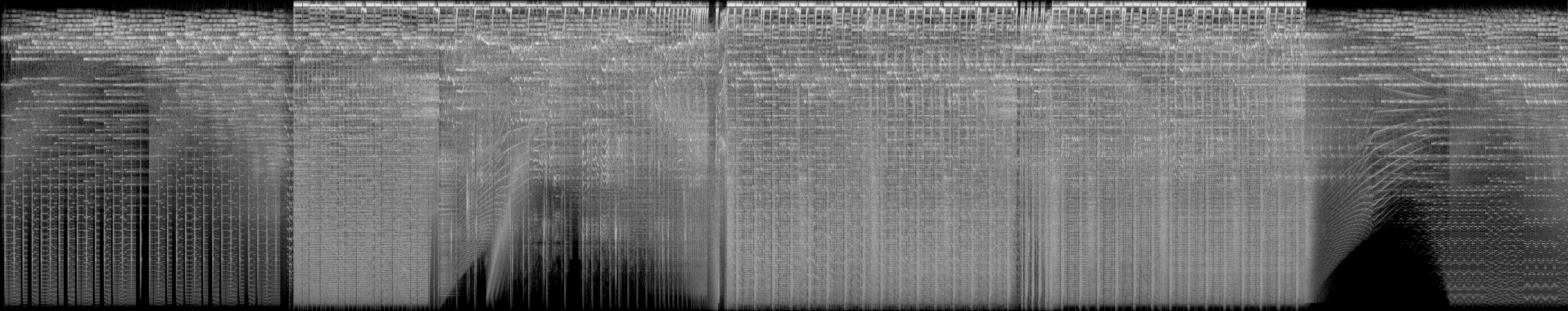
Sound is really just waves of pressure through the air, and the audio files we play are digital recordings of how the air pressure changes over time. However, human ears do not directly detect the air pressure. Instead, the ear contains many hairs each detect sound waves of a particular frequency, and the sum of these vibrations is what we hear. Because the program is trying to classify sound according to human characteristics, it makes sense to transform the input features into what humans percieve. This can be done by using the audio signal to creating a spectrogram, which display how intense the vibrations of each frequency are at each point in time.
Next, the data can be classified using artificial intelligence. Convolutional neural networks are a suitable model for this purpose, for the following reasons
- The input will be a 2 dimensional spectrogram
- The data should be continuous, as the intensity of two points very close in time or frequency should be nearly the same
- playing the entire song earlier or later in time does not affect how we percieve the song
- shifting the frequency of the song by a small amount is also unlikely to affect the listening experience
The model will be built in Python using Pytorch.
Obtaining Data
Fortunately, my friend already had a library of about 1000 songs. Also, Youtube kept a convenient history of all previously listened songs. So using yt-dlp, I downloaded the full library and about 3000 songs from the history.
Cleaning data
Some of the files were podcasts, song/album compilations, and other undesirable data. Luckily, almost all songs had the song title and author provided in the file metadata, so I simply deleted the files without it. I also removed duplicate files with the same title and author, and deleted audio shorter than 1 minute or longer than 5 minutes. Finally, based on the filename (title and author also works), I removed songs from the full history that also appeared in the set of good songs, and chose about 1000 random remaining songs to be the ‘bad’ dataset.
Processing data
All of the files are then converted to 48khz .wav format using ffmpeg. Since wav files do not have compression, the encoding process is very fast.
The files get placed in the ‘data’ folder, sorted by their classification. In this case, the folders are data/good/ and data/bad/.
Processing data part 2
Next, the data will be converted into spectrograms. Pytorch as
First, the data is loaded. At this point, the dataset was over 70GB, much more than the memory on my system. So only filename and classification are stored, while the audio signial will be loaded as needed.
import os
import torch
import torchaudio
from torchaudio import transforms
import matplotlib.pyplot as plt
from torch.utils.data import Dataset, DataLoader
from pathlib import Path
import math,random
from IPython.display import Audio

#load data
def load_audio_files(path: str, label:str):

    dataset = []
    walker = sorted(str(p) for p in Path(path).glob(f'*.wav'))

    for i, file_path in enumerate(walker):
        path, filename = os.path.split(file_path)

        # Load audio
        #waveform, sample_rate = torchaudio.load(file_path)
        dataset.append([file_path, label])

    return dataset

trainset_music_good = load_audio_files('./data/good', 'good')
trainset_music_bad = load_audio_files('./data/bad', 'bad')
trainset_music=trainset_music_good+trainset_music_bad
The audio for each file is read, converted to single channel, and truncated to 2 minutes (if it is shorter than 2 minutes, it is padded with silence). This is so all the inputs have the same shape, and listening to 2 minutes of a song should be enough to form an opinion on it (my guess). Next, it is converted to a spectrogram. Humans percieve pitch and loudness on a logarithmic scale (for example, doubling a music note increases it by one octave), so a mel spectrogram with a decibel scale is used.
def open_file(audio_file):
    waveform, sample_rate = torchaudio.load(audio_file)
    return (waveform, sample_rate)

#convert stereo to mono to save resources
def toMono(audio):
    waveform,s=audio
    return (waveform[:1,:],s)

def pad_trunc(aud, max_ms):
    sig, sr = aud
    num_rows, sig_len = sig.shape
    max_len = sr//1000 * max_ms

    if (sig_len > max_len):
        # Truncate the signal to the given length
        sig = sig[:,:max_len]

    elif (sig_len < max_len):
        # Length of padding to add at the beginning and end of the signal
        pad_begin_len = random.randint(0, max_len - sig_len)
        pad_end_len = max_len - sig_len - pad_begin_len

        # Pad with 0s
        pad_begin = torch.zeros((num_rows, pad_begin_len))
        pad_end = torch.zeros((num_rows, pad_end_len))

        sig = torch.cat((pad_begin, sig, pad_end), 1)

    return (sig, sr)

def spectro_gram(aud, n_mels=512, n_fft=4096, hop_len=None):
    sig,sr = aud
    top_db = 80

    # spec has shape [channel, n_mels, time], where channel is mono, stereo etc
    spec = transforms.MelSpectrogram(sr, n_fft=n_fft, hop_length=hop_len, n_mels=n_mels)(sig)

    # Convert to decibels
    spec = transforms.AmplitudeToDB(top_db=top_db)(spec)
    return (spec)


for data in trainset_music:
    filename=data[0]

    wv=open_file(filename)
    wv=toMono(wv)
    wv=pad_trunc(wv,60000*2)

    spec=spectro_gram(wv)
    spec=spec[0].detach().numpy()

    label=data[1]

    _,filename=os.path.split(filename)
    filename,_=os.path.splitext(filename)

    plt.imsave(f'./data/spectrograms/{label}/{filename}.png',spec,cmap='gray')
This conversion took over an hour on my computer. The resulting spectrogram is saved as a file so it does not have to be recalculated every time I train the model.
Training
The spectrograms are converted back from an image file to a tensor and loaded into a training and testing dataset, with 80% used for training.
data_path = './data/spectrograms' #looking in subfolder train
dataset = datasets.ImageFolder(root=data_path,transform=transforms.Compose([transforms.Grayscale(),transforms.ToTensor()]))
class_map=dataset.class_to_idx
print(class_map)

#split data to test and train
#use 80% to train
train_size = int(0.8 * len(dataset))
test_size = len(dataset) - train_size
train_dataset, test_dataset = torch.utils.data.random_split(dataset, [train_size, test_size])

print("Training size:", len(train_dataset))
print("Testing size:",len(test_dataset))

train_dataloader = torch.utils.data.DataLoader(
    train_dataset,
    batch_size=15,
    num_workers=2,
    shuffle=True
)

test_dataloader = torch.utils.data.DataLoader(
    test_dataset,
    batch_size=50,
    num_workers=2,
    shuffle=True
)
print(torch.cuda.is_available())
Now it is time to build the model. Initially, I used 4 convolutional layers followed by 2 dense layers.
Compared to image object classification I’ve done before, the spectrograms are very high resolution. I do not want to reduce the initial resolution because it could destroy a lot of data in the sound timbre, and in addition music can sound very bad if the notes are a semitone off (but it’s just my thought process, I am not an expert in sound).
Instead, I used max pooling after the convolutional layers where it has hopefully already extracted the important features.
class CNNet (nn.Module):
    # ----------------------------
    # Build the model architecture
    # ----------------------------
    def __init__(self):
        super().__init__()
        conv_layers = []

        # First Convolution Block with Relu and Batch Norm. Use Kaiming Initialization
        self.conv1 = nn.Conv2d(1, 8, kernel_size=5)
        self.relu1 = nn.ReLU()
        self.bn1 = nn.BatchNorm2d(8)
        nn.init.kaiming_normal_(self.conv1.weight, a=0.1)
        self.conv1.bias.data.zero_()
        conv_layers += [self.conv1, self.relu1,self.bn1]

        # Second Convolution Block
        self.conv2 = nn.Conv2d(8, 16, kernel_size=3)
        self.relu2 = nn.ReLU()
        self.bn2 = nn.BatchNorm2d(16)
        nn.init.kaiming_normal_(self.conv2.weight, a=0.1)
        self.conv2.bias.data.zero_()
        self.drop2 = nn.Dropout2d()
        self.pool2=nn.MaxPool2d(2)
        conv_layers += [self.conv2, self.pool2, self.relu2,self.bn2]

        # third Convolution Block
        self.conv3 = nn.Conv2d(16, 32, kernel_size=3)
        self.relu3 = nn.ReLU()
        self.bn3 = nn.BatchNorm2d(32)
        nn.init.kaiming_normal_(self.conv3.weight, a=0.1)
        self.conv3.bias.data.zero_()
        self.drop3 = nn.Dropout2d()
        self.pool3=nn.MaxPool2d(2)
        conv_layers += [self.conv3, self.drop3, self.pool3,self.relu3,self.bn3]

        # fourth Convolution Block
        self.conv4 = nn.Conv2d(32, 64, kernel_size=3)
        self.relu4 = nn.ReLU()
        self.bn4 = nn.BatchNorm2d(64)
        nn.init.kaiming_normal_(self.conv4.weight, a=0.1)
        self.conv4.bias.data.zero_()
        self.drop4 = nn.Dropout2d()
        self.pool4=nn.MaxPool2d(2)
        conv_layers += [self.conv4, self.drop4, self.pool4,self.relu4,self.bn4]

        # 5 Block
        self.conv5 = nn.Conv2d(64, 64, kernel_size=3)
        self.relu5 = nn.ReLU()
        self.bn5 = nn.BatchNorm2d(64)
        nn.init.kaiming_normal_(self.conv5.weight, a=0.1)
        self.conv5.bias.data.zero_()
        self.drop5 = nn.Dropout2d()
        self.pool5=nn.MaxPool2d(2)
        conv_layers += [self.conv5, self.drop5, self.pool5,self.relu5,self.bn5]

        # Block 6
        self.conv6 = nn.Conv2d(64, 64, kernel_size=3, stride=(2, 2))
        self.relu6 = nn.ReLU()
        self.bn6 = nn.BatchNorm2d(64)
        nn.init.kaiming_normal_(self.conv6.weight, a=0.1)
        self.conv6.bias.data.zero_()
        self.drop6 = nn.Dropout2d()
        self.pool6=nn.MaxPool2d(2)
        conv_layers += [self.conv6, self.drop6, self.pool6,self.relu6,self.bn6]

        self.flatten=nn.Flatten()
        # Linear Classifier
        self.lin1 = nn.Linear(19264,50)
        self.lin2=nn.Linear(50,2)

        # Wrap the Convolutional Blocks
        self.conv = nn.Sequential(*conv_layers)

    # ----------------------------
    # Forward pass computations
    # ----------------------------
    def forward(self, x):
        # Run the convolutional blocks
        x = self.conv(x)

        # Adaptive pool and flatten for input to linear layer
        x = x.view(x.shape[0], -1)
        x=self.flatten(x)

        # Linear layer
        x = F.relu(self.lin1(x))
        x=self.lin2(x)

        # Final output
        x=F.log_softmax(x,dim=1)
        return x

# Create the model and put it on the GPU if available
myModel = CNNet()
device = torch.device("cuda:0" if torch.cuda.is_available() else "cpu")
myModel = myModel.to(device)
# Check that it is on Cuda
next(myModel.parameters()).device

summary(myModel, input_size=(25,1,2813,512))
Training took about 30 minutes on my single Nvidia RTX 3090:
# cost function used to determine best parameters
cost = torch.nn.CrossEntropyLoss()

# used to create optimal parameters
learning_rate = 0.0001
optimizer = torch.optim.Adam(myModel.parameters(), lr=learning_rate)

# Create the training function

def train(dataloader, model, loss, optimizer):
    model.train()
    size = len(dataloader.dataset)
    for batch, (X, Y) in enumerate(dataloader):

        X, Y = X.to(device), Y.to(device)
        optimizer.zero_grad()
        pred = model(X)
        loss = cost(pred, Y)
        loss.backward()
        optimizer.step()

        if batch % 60 == 0:
            loss, current = loss.item(), batch * len(X)
            print(f'loss: {loss:>7f}  [{current:>5d}/{size:>5d}]')


# Create the validation/test function

def test(dataloader, model):
    model.eval()
    test_loss, correct = 0, 0

    with torch.no_grad():
        for batch, (X, Y) in enumerate(dataloader):
            X, Y = X.to(device), Y.to(device)
            pred = model(X)

            test_loss += cost(pred, Y).item()
            correct += (pred.argmax(1)==Y).type(torch.float).sum().item()

    test_loss /= len(dataloader)
    correct /= len(dataloader.dataset)

    print(f'\nTest Error:\nacc: {(100*correct):>0.1f}%, avg loss: {test_loss:>8f}\n')

#training
epochs = 15

for t in range(epochs):
    print(f'Epoch {t+1}\n-------------------------------')
    train(train_dataloader, myModel, cost, optimizer)
    test(test_dataloader, myModel)
print('Done!')
The training loss quickly approached 0, but the the testing loss did not decrease significantly. At the end, the model had 60% accuracy, barely better than random guessing. So it was clearly overfitting.
I added a dropout layer after every convolutional layer other than the first, and reran the training. This time, the training loss fluctuated highly and sometimes even increased. In the end, both the training and testing performance were not great. This was fixed by decreasing the learning rate and increasing the number of training epochs to 25, by which point the process significant slowed down.
I then added more convolutional layers and decreased the learning rate. I also decided to increase the dataset through data augmentation.
def open_file(audio_file):
    waveform, sample_rate = torchaudio.load(audio_file)
    return (waveform, sample_rate)

#convert stereo to mono to save resources
def toMono(audio):
    waveform,s=audio
    return (waveform[:1,:],s)

def pad_trunc(aud, max_ms):
    sig, sr = aud
    num_rows, sig_len = sig.shape
    max_len = sr//1000 * max_ms

    if (sig_len > max_len):
        # Truncate the signal to the given length
        sig = sig[:,:max_len]

    elif (sig_len < max_len):
        # Length of padding to add at the beginning and end of the signal
        pad_begin_len = random.randint(0, max_len - sig_len)
        pad_end_len = max_len - sig_len - pad_begin_len

        # Pad with 0s
        pad_begin = torch.zeros((num_rows, pad_begin_len))
        pad_end = torch.zeros((num_rows, pad_end_len))

        sig = torch.cat((pad_begin, sig, pad_end), 1)

    return (sig, sr)

def time_shift(aud, shift_limit):
    sig,sr = aud
    _, sig_len = sig.shape
    shift_amt = int(random.random() * shift_limit * sig_len)
    return (sig.roll(shift_amt), sr)

def pitch_shift(aud, shift_limit):
    sig,sr = aud
    shift_amt = int(random.random() * shift_limit)
    sig=transforms.PitchShift(sample_rate=sr, n_steps=shift_amt)(sig)
    return (sig,sr)
def speed_shift(aud, shift_limit):
    sig,sr = aud
    shift_amt = int(random.random() * shift_limit)
    sig=transforms.Speed(sig,sr, shift_amt)
    return (sig,sr)

def data_augment(aud):
    aud=pitch_shift(aud,4)
    aud=time_shift(aud,0.1)
    return aud
def stretch(spec):
    rate=int(random.random()*0.2)+0.9
    spec=transforms.TimeStretch(n_freq=512,fixed_rate=rate)(spec)
    return spec

def spectro_gram(aud, n_mels=512, n_fft=4096, hop_len=None):
    sig,sr = aud
    top_db = 80

    # spec has shape [channel, n_mels, time], where channel is mono, stereo etc
    spec = transforms.MelSpectrogram(sr, n_fft=n_fft, hop_length=hop_len, n_mels=n_mels)(sig)

    # Convert to decibels
    spec = transforms.AmplitudeToDB(top_db=top_db)(spec)
    return (spec)


for i in range(0,3):
    for data in trainset_music:
        filename=data[0]

        wv=open_file(filename)
        wv=toMono(wv)
        wv=pad_trunc(wv,60000*2)
        if i>0:
            wv=data_augment(wv)
        spec=spectro_gram(wv)
        spec=spec[0].detach().numpy()

        label=data[1]

        _,filename=os.path.split(filename)
        filename,_=os.path.splitext(filename)

        plt.imsave(f'./data/spectrograms/{label}/{filename}_{i}.png',spec,cmap='gray')
There are several ways to augment audio data. First, the audio can be simply shifted in time. The pitch can be slightly adjusted up or down, and the song can be sped up or slowed down by a small factor. For each song, I added two more datapoints by applying a random combination of these 3 transformations.
After these changes, the model finally began learning again. For my final attempt, I increase the training epochs to 50. After training for 2.5 hours, it had a test accuracy of about 88%.
Prediction
#predictions
def predict(data, model):
    model.eval()
    test_loss, correct = 0, 0
    with torch.no_grad():
        for filename,(X, Y) in zip(data.imgs,data):
            X.unsqueeze_(-1)
            X=X.transpose(1,3)
            X=X.to(device)
            pred = model(X)
            pred=pred.argmax(1)
            print(filename,reverse_class_map[pred])


#convert to spectrogram first using data_prep
inference_dataset = datasets.ImageFolder(root='./data/test/',transform=transforms.Compose([transforms.Grayscale(),transforms.ToTensor()]))
predict(inference_dataset,myModel)
Conclusion
It’s possible that one’s taste in music has changed over time, so the earlier datapoints were harmful to the training.
Unfortunately the performance is not as great as I was used to on more standard CNN tasks such as MNIST. In addition, it required a large collection of labeled data on my friend’s music preferences, which many people may not have. Still, after downloading and using the model to filter through some new songs (and listening the remaining ones myself) them I was able make several recommendations my friend enjoyed.
Retraining for other tasks
Since I already had all the code written, I wanted to see if the same model could be retrained to work for other sound classification tasks. This time, I found and downloaded a playlist of classical music and electronic music. The audio was again converted to spectrograms, without data augmentation. I then retrained the model on this data, and it had an accuracy of 99.7%. So that was definitely a success.